Example_tasks
[2]:
# import datacleanbot and openml
import datacleanbot.dataclean as dc
import openml as oml
import numpy as np
Preparation: Acquire Data
The first step is to acquire data from OpneML. The dataset ID can be found in the address.
[3]:
# acquire dataset with dataset ID 4
data = oml.datasets.get_dataset(4)
X, y, categorical_indicator, features = data.get_data(target=data.default_target_attribute, dataset_format='array')
Xy = np.concatenate((X,y.reshape((y.shape[0],1))), axis=1)
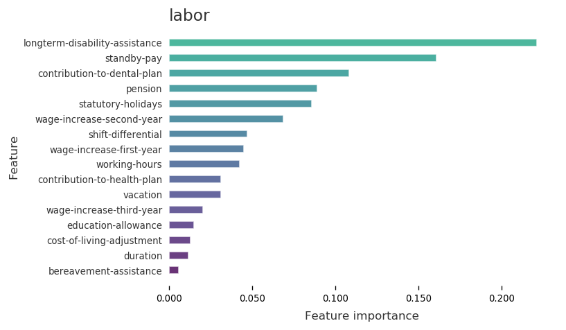
Task 1: Show Important Features
[4]:
dc.show_important_features(X, y, data.name, features)
Important Features
Task 2: Unify Column Names
[5]:
features = dc.unify_name_consistency(features)
Inconsitent Column Names
Column names
============
['duration', 'wage-increase-first-year', 'wage-increase-second-year', 'wage-increase-third-year', 'cost-of-living-adjustment', 'working-hours', 'pension', 'standby-pay', 'shift-differential', 'education-allowance', 'statutory-holidays', 'vacation', 'longterm-disability-assistance', 'contribution-to-dental-plan', 'bereavement-assistance', 'contribution-to-health-plan']

Column names are consistent
Task 3: Show Statistical Information
[6]:
dc.show_statistical_info(Xy)
Statistical Information
| 0 | 1 | 2 | 3 | 4 | 5 | 6 | 7 | 8 | 9 | 10 | 11 | 12 | 13 | 14 | 15 | 16 | |
|---|---|---|---|---|---|---|---|---|---|---|---|---|---|---|---|---|---|
| count | 30.000000 | 37.000000 | 37.000000 | 37.000000 | 56.000000 | 22.000000 | 28.000000 | 27.000000 | 31.000000 | 9.000000 | 53.000000 | 51.000000 | 56.000000 | 46.000000 | 15.000000 | 51.000000 | 57.000000 |
| mean | 0.100000 | 1.108108 | 1.324324 | 0.594595 | 2.160714 | 0.545455 | 0.285714 | 1.037037 | 4.870968 | 7.444444 | 11.094340 | 0.960784 | 3.803571 | 3.971739 | 3.913333 | 38.039216 | 0.649123 |
| std | 0.305129 | 0.774015 | 0.818333 | 0.797895 | 0.707795 | 0.509647 | 0.460044 | 0.939782 | 4.544168 | 5.027701 | 1.259795 | 0.823669 | 1.370596 | 1.164028 | 1.304315 | 2.505680 | 0.481487 |
| min | 0.000000 | 0.000000 | 0.000000 | 0.000000 | 1.000000 | 0.000000 | 0.000000 | 0.000000 | 0.000000 | 2.000000 | 9.000000 | 0.000000 | 2.000000 | 2.000000 | 2.000000 | 27.000000 | 0.000000 |
| 25% | 0.000000 | 1.000000 | 1.000000 | 0.000000 | 2.000000 | 0.000000 | 0.000000 | 0.000000 | 3.000000 | 2.000000 | 10.000000 | 0.000000 | 2.500000 | 3.000000 | 2.400000 | 37.000000 | 0.000000 |
| 50% | 0.000000 | 1.000000 | 2.000000 | 0.000000 | 2.000000 | 1.000000 | 0.000000 | 1.000000 | 4.000000 | 8.000000 | 11.000000 | 1.000000 | 4.000000 | 4.000000 | 4.600000 | 38.000000 | 1.000000 |
| 75% | 0.000000 | 2.000000 | 2.000000 | 1.000000 | 3.000000 | 1.000000 | 1.000000 | 2.000000 | 5.000000 | 12.000000 | 12.000000 | 2.000000 | 4.500000 | 4.500000 | 5.000000 | 40.000000 | 1.000000 |
| max | 1.000000 | 2.000000 | 2.000000 | 2.000000 | 3.000000 | 1.000000 | 1.000000 | 2.000000 | 25.000000 | 14.000000 | 15.000000 | 2.000000 | 7.000000 | 7.000000 | 5.100000 | 40.000000 | 1.000000 |
Task 4: Discover Data Types
[7]:
# input can be Xy or X
dc.discover_types(Xy)
Discover Data Types
Simple Data Types
['float64', 'int64', 'float64', 'int64', 'int64', 'int64', 'float64', 'int64', 'int64', 'float64', 'int64', 'int64', 'float64', 'float64', 'float64', 'int64', 'bool']
Statistical Data Types
['Type.POSITIVE', 'Type.REAL', 'Type.REAL', 'Type.POSITIVE', 'Type.POSITIVE', 'Type.POSITIVE', 'Type.POSITIVE', 'Type.POSITIVE', 'Type.POSITIVE', 'Type.POSITIVE', 'Type.POSITIVE', 'Type.REAL', 'Type.POSITIVE', 'Type.POSITIVE', 'Type.REAL', 'Type.POSITIVE', 'Type.COUNT']
Task 5: Clean Duplicated Rows
[8]:
Xy = dc.clean_duplicated_rows(Xy)
Duplicated Rows
Identifying Duplicated Rows ...
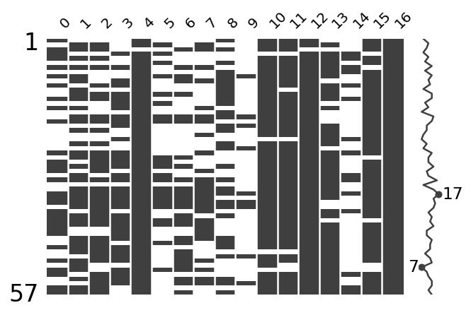
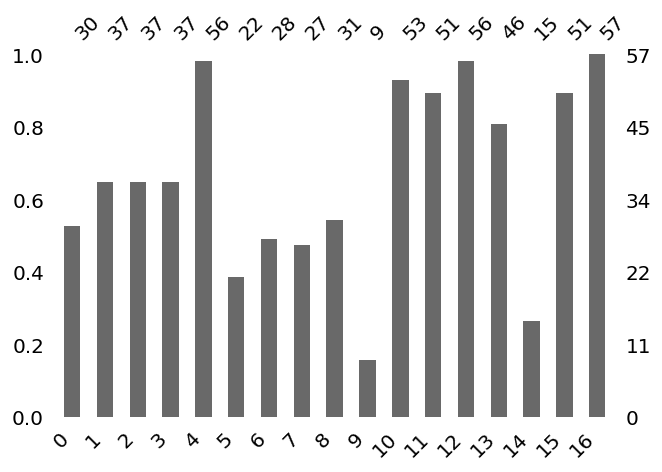
Task 6: Handle Missing Values
[9]:
features, Xy = dc.handle_missing(features, Xy)
Missing values
Identify Missing Data ...
The default setting of missing characters is ['n/a', 'na', '--', '?']
Do you want to add extra character? [y/n]n
Number of missing in each feature
0     27
1     20
2     20
3     20
4      1
5     35
6     29
7     30
8     26
9     48
10     4
11     6
12     1
13    11
14    42
15     6
16     0
dtype: int64

Records containing missing values:
| 0 | 1 | 2 | 3 | 4 | 5 | 6 | 7 | 8 | 9 | 10 | 11 | 12 | 13 | 14 | 15 | 16 | |
|---|---|---|---|---|---|---|---|---|---|---|---|---|---|---|---|---|---|
| 0 | 0.0 | NaN | NaN | NaN | 1.0 | NaN | NaN | NaN | 2.0 | NaN | 11.0 | 1.0 | 5.0 | NaN | NaN | 40.0 | 1.0 |
| 1 | NaN | 2.0 | 2.0 | NaN | 2.0 | 0.0 | NaN | 1.0 | NaN | NaN | 11.0 | 0.0 | 4.5 | 5.8 | NaN | 35.0 | 1.0 |
| 2 | 0.0 | 1.0 | 1.0 | NaN | NaN | NaN | 0.0 | 2.0 | 5.0 | NaN | 11.0 | 2.0 | NaN | NaN | NaN | 38.0 | 1.0 |
| 3 | 0.0 | NaN | NaN | 2.0 | 3.0 | 0.0 | NaN | NaN | NaN | NaN | NaN | NaN | 3.7 | 4.0 | 5.0 | NaN | 1.0 |
| 4 | 0.0 | 1.0 | 1.0 | NaN | 3.0 | NaN | NaN | NaN | NaN | NaN | 12.0 | 1.0 | 4.5 | 4.5 | 5.0 | 40.0 | 1.0 |
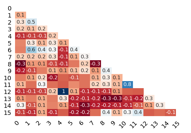
Missing correlation between features containing missing values and other features
| 0 | 1 | 2 | 3 | 4 | 5 | 6 | 7 | 8 | 9 | 10 | 11 | 12 | 13 | 14 | 15 | |
|---|---|---|---|---|---|---|---|---|---|---|---|---|---|---|---|---|
| 0 | 1.000000 | 0.112373 | 0.259620 | 0.185996 | -0.126773 | 0.030389 | 0.018496 | 0.196296 | -0.304456 | -0.167360 | 0.014479 | 0.132569 | -0.126773 | 0.070290 | 0.327569 | -0.096414 |
| 1 | 0.112373 | 1.000000 | 0.460811 | 0.152703 | -0.098247 | 0.280850 | 0.575362 | 0.182121 | 0.064742 | -0.084895 | 0.085841 | -0.012609 | -0.098247 | 0.013074 | -0.061512 | -0.132393 |
| 2 | 0.259620 | 0.460811 | 1.000000 | 0.229730 | -0.098247 | 0.129827 | 0.428296 | 0.182121 | 0.064742 | 0.015918 | 0.229751 | 0.346743 | -0.098247 | 0.106224 | 0.105450 | 0.107175 |
| 3 | 0.185996 | 0.152703 | 0.229730 | 1.000000 | 0.181757 | 0.280850 | 0.354763 | 0.255745 | -0.082870 | 0.116731 | -0.201979 | -0.012609 | 0.181757 | 0.013074 | 0.021969 | -0.132393 |
| 4 | -0.126773 | -0.098247 | -0.098247 | 0.181757 | 1.000000 | 0.105946 | -0.135996 | -0.140859 | -0.122380 | 0.057864 | -0.036711 | -0.045835 | 1.000000 | 0.273268 | 0.079860 | -0.045835 |
| 5 | 0.030389 | 0.280850 | 0.129827 | 0.280850 | 0.105946 | 1.000000 | 0.374342 | 0.113961 | 0.002539 | 0.150845 | -0.064352 | 0.037082 | 0.105946 | -0.160206 | -0.146448 | -0.197772 |
| 6 | 0.018496 | 0.575362 | 0.428296 | 0.354763 | -0.135996 | 0.374342 | 1.000000 | 0.332923 | 0.195304 | 0.248198 | -0.004820 | -0.006018 | -0.135996 | -0.141967 | -0.268444 | -0.234718 |
| 7 | 0.196296 | 0.182121 | 0.182121 | 0.255745 | -0.140859 | 0.113961 | 0.332923 | 1.000000 | -0.259902 | 0.071001 | 0.123072 | 0.210905 | -0.140859 | -0.159324 | -0.167984 | -0.018078 |
| 8 | -0.304456 | 0.064742 | 0.064742 | -0.082870 | -0.122380 | 0.002539 | 0.195304 | -0.259902 | 1.000000 | 0.396558 | 0.299976 | 0.259754 | -0.122380 | -0.269331 | -0.172611 | 0.374528 |
| 9 | -0.167360 | -0.084895 | 0.015918 | 0.116731 | 0.057864 | 0.150845 | 0.248198 | 0.071001 | 0.396558 | 1.000000 | 0.118958 | 0.148522 | 0.057864 | -0.275913 | -0.149514 | 0.148522 |
| 10 | 0.014479 | 0.085841 | 0.229751 | -0.201979 | -0.036711 | -0.064352 | -0.004820 | 0.123072 | 0.299976 | 0.118958 | 1.000000 | 0.800943 | -0.036711 | -0.134341 | -0.147760 | 0.353357 |
| 11 | 0.132569 | -0.012609 | 0.346743 | -0.012609 | -0.045835 | 0.037082 | -0.006018 | 0.210905 | 0.259754 | 0.148522 | 0.800943 | 1.000000 | -0.045835 | -0.167729 | -0.054661 | 0.441176 |
| 12 | -0.126773 | -0.098247 | -0.098247 | 0.181757 | 1.000000 | 0.105946 | -0.135996 | -0.140859 | -0.122380 | 0.057864 | -0.036711 | -0.045835 | 1.000000 | 0.273268 | 0.079860 | -0.045835 |
| 13 | 0.070290 | 0.013074 | 0.106224 | 0.013074 | 0.273268 | -0.160206 | -0.141967 | -0.159324 | -0.269331 | -0.275913 | -0.134341 | -0.167729 | 0.273268 | 1.000000 | 0.292239 | -0.022872 |
| 14 | 0.327569 | -0.061512 | 0.105450 | 0.021969 | 0.079860 | -0.146448 | -0.268444 | -0.167984 | -0.172611 | -0.149514 | -0.147760 | -0.054661 | 0.079860 | 0.292239 | 1.000000 | -0.054661 |
| 15 | -0.096414 | -0.132393 | 0.107175 | -0.132393 | -0.045835 | -0.197772 | -0.234718 | -0.018078 | 0.374528 | 0.148522 | 0.353357 | 0.441176 | -0.045835 | -0.022872 | -0.054661 | 1.000000 |
Visualize Missing Data ...
Clean Missing Data ...
Choose the missing mechanism [a/b/c/d]:
a.MCAR b.MAR c.MNAR d.Skip
a
Missing percentage is 0.9824561403508771
Imputation score of mean is 0.8515151515151516
Imputation score of mode is 0.8674242424242424
Imputation score of knn is 0.9299242424242424
Imputation score of matrix factorization is 0.9299242424242424
Imputation score of multiple imputation is 0.9291666666666667
Imputation method with the highest socre is knn
The recommended approach is knn
Do you want to apply the recommended approach? [y/n]n


Choose the approach you want to apply [a/b/c/d/e/skip]:
a.Mean b.Mode c.K Nearest Neighbor d.Matrix Factorization e. Multiple Imputation
a

Applying mean imputation ...
Missing values cleaned!
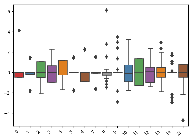
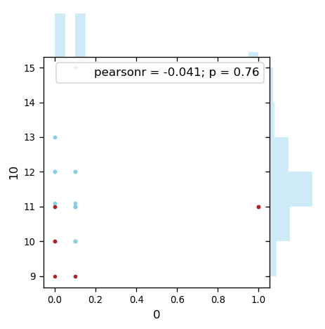
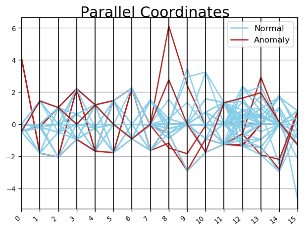
Task 7: Handle Outliers
[10]:
Xy = dc.handle_outlier(features,Xy)
Outliers
Recommend Algorithm ...
The recommended approach is isolation forest.
Do you want to apply the recommended outlier detection approach? [y/n]y
Visualize Outliers ...
| 0 | 1 | 2 | 3 | 4 | 5 | 6 | 7 | 8 | 9 | 10 | 11 | 12 | 13 | 14 | 15 | 16 | anomaly_score | |
|---|---|---|---|---|---|---|---|---|---|---|---|---|---|---|---|---|---|---|
| 36 | 1 | 0 | 0 | 2 | 1 | 1 | 1 | 1 | 0 | 4 | 11 | 2 | 2 | 3.97174 | 3.91333 | 40 | 0 | -0.0883411 |
| 34 | 0 | 1 | 2 | 2 | 3 | 1 | 1 | 0 | 1 | 2 | 10 | 0 | 2 | 2.5 | 2.1 | 40 | 0 | -0.0724028 |
| 40 | 1 | 0 | 0 | 0 | 1 | 0 | 1 | 0 | 4.87097 | 7.44444 | 11 | 1 | 4 | 3.97174 | 3.91333 | 38.0392 | 0 | -0.0318737 |
| 18 | 1 | 0 | 0 | 0 | 1 | 0 | 1 | 0 | 4.87097 | 7.44444 | 11 | 1 | 2 | 3.97174 | 3.91333 | 38 | 0 | -0.0313807 |
| 56 | 0 | 2 | 2 | 0.594595 | 3 | 0.545455 | 0 | 1.03704 | 14 | 7.44444 | 9 | 2 | 6 | 6 | 4 | 35 | 1 | -0.0218354 |
| 8 | 0 | 1 | 1.32432 | 0.594595 | 2 | 0 | 0 | 1.03704 | 25 | 12 | 11 | 0 | 3 | 7 | 3.91333 | 38 | 1 | -0.0199344 |
| 17 | 0.1 | 1 | 0 | 2 | 1 | 1 | 0 | 1 | 3 | 2 | 9 | 0 | 2.1 | 3.97174 | 3.91333 | 40 | 0 | -0.0124747 |
| 31 | 0 | 1 | 2 | 2 | 3 | 1 | 0 | 0 | 5 | 7.44444 | 10 | 0 | 3 | 2 | 2.5 | 40 | 0 | -0.00911494 |
| 6 | 0 | 0 | 1 | 2 | 3 | 0.545455 | 0 | 2 | 4.87097 | 7.44444 | 12 | 2 | 4 | 5 | 5 | 38.0392 | 1 | -0.00885507 |
| 37 | 0.1 | 1 | 0 | 0 | 1 | 1 | 0 | 2 | 3 | 2 | 9 | 0 | 2.8 | 3.97174 | 3.91333 | 38 | 0 | -0.00362979 |
| 38 | 0 | 1.10811 | 0 | 0.594595 | 3 | 0.545455 | 0.285714 | 2 | 4.87097 | 7.44444 | 10 | 1 | 2 | 2.5 | 2 | 37 | 0 | 0.00190097 |
| 25 | 0 | 1 | 2 | 0 | 3 | 0.545455 | 0.285714 | 0 | 4.87097 | 7.44444 | 10 | 0 | 2 | 2 | 2 | 40 | 0 | 0.00266917 |
| 33 | 0.1 | 0 | 0 | 0 | 2 | 1 | 1 | 0 | 3 | 7.44444 | 10 | 0 | 4 | 5 | 3.91333 | 40 | 0 | 0.00353423 |
| 41 | 0 | 0 | 2 | 0 | 2 | 0 | 0 | 2 | 4.87097 | 7.44444 | 12 | 2 | 2 | 3 | 3.91333 | 38 | 0 | 0.0133322 |
| 35 | 0 | 0 | 2 | 0 | 2 | 1 | 0 | 0 | 4.87097 | 7.44444 | 11 | 1 | 2 | 2 | 3.91333 | 40 | 0 | 0.0134714 |
| 19 | 0.1 | 1.10811 | 1.32432 | 1 | 2 | 0.545455 | 0.285714 | 1.03704 | 5 | 13 | 15 | 2 | 4 | 5 | 3.91333 | 35 | 1 | 0.0161718 |
| 7 | 0.1 | 1.10811 | 1.32432 | 0.594595 | 3 | 0.545455 | 0.285714 | 1.03704 | 3 | 7.44444 | 12 | 0 | 6.9 | 4.8 | 2.3 | 40 | 1 | 0.0208748 |
| 11 | 0.1 | 2 | 1.32432 | 0.594595 | 2 | 0.545455 | 0.285714 | 1.03704 | 4 | 7.44444 | 15 | 0.960784 | 6.4 | 6.4 | 3.91333 | 38 | 1 | 0.0243395 |
| 14 | 0.1 | 1.10811 | 1.32432 | 0 | 1 | 1 | 0.285714 | 1.03704 | 10 | 7.44444 | 11 | 2 | 3 | 3.97174 | 3.91333 | 36 | 1 | 0.0247281 |
| 9 | 0.1 | 2 | 1.32432 | 0 | 1 | 0.545455 | 0 | 2 | 4 | 7.44444 | 11 | 2 | 5.7 | 3.97174 | 3.91333 | 40 | 1 | 0.0269993 |
| 44 | 0.1 | 0 | 0 | 0 | 2 | 0.545455 | 1 | 0 | 3 | 7.44444 | 10 | 0 | 4 | 4 | 3.91333 | 40 | 0 | 0.0270557 |
| 27 | 0 | 1.10811 | 2 | 0 | 2 | 0 | 0.285714 | 1.03704 | 4.87097 | 7.44444 | 12 | 2 | 3 | 3 | 3.91333 | 33 | 1 | 0.0310571 |
| 13 | 0 | 2 | 2 | 1 | 3 | 0.545455 | 0.285714 | 1.03704 | 4 | 7.44444 | 13 | 2 | 3.5 | 4 | 5.1 | 37 | 1 | 0.0398261 |
| 26 | 0.1 | 0 | 1 | 1 | 2 | 0 | 0 | 1.03704 | 4.87097 | 7.44444 | 10 | 0 | 4.5 | 4.5 | 3.91333 | 38.0392 | 1 | 0.0399781 |
| 29 | 0 | 1.10811 | 2 | 0.594595 | 3 | 0.545455 | 0.285714 | 0 | 4.87097 | 7.44444 | 10 | 1 | 2 | 2.5 | 3.91333 | 35 | 0 | 0.0402457 |
| 53 | 0.1 | 2 | 2 | 0 | 3 | 0.545455 | 0 | 2 | 6 | 7.44444 | 11 | 1 | 4 | 3.5 | 3.91333 | 40 | 1 | 0.0404225 |
| 42 | 0 | 1.10811 | 1.32432 | 2 | 2 | 0.545455 | 0.285714 | 2 | 4.87097 | 7.44444 | 12 | 1 | 2.5 | 2.5 | 3.91333 | 39 | 0 | 0.0435786 |
| 54 | 0.1 | 1.10811 | 2 | 0 | 3 | 0.545455 | 0 | 2 | 6 | 10 | 11 | 2 | 5 | 4.4 | 3.91333 | 38 | 1 | 0.0459069 |
| 1 | 0.1 | 2 | 2 | 0.594595 | 2 | 0 | 0.285714 | 1 | 4.87097 | 7.44444 | 11 | 0 | 4.5 | 5.8 | 3.91333 | 35 | 1 | 0.0467527 |
| 24 | 0.1 | 1.10811 | 1.32432 | 0.594595 | 1 | 0.545455 | 0.285714 | 1.03704 | 3 | 8 | 9 | 2 | 6 | 3.97174 | 3.91333 | 38 | 1 | 0.0475632 |
| 51 | 0 | 1 | 1.32432 | 1 | 3 | 0 | 0 | 2 | 4.87097 | 7.44444 | 11.0943 | 0.960784 | 2 | 3 | 3.91333 | 38.0392 | 1 | 0.0477415 |
| 28 | 0 | 2 | 2 | 0 | 2 | 1 | 0 | 1.03704 | 5 | 7.44444 | 11 | 0 | 5 | 4 | 3.91333 | 37 | 1 | 0.0485515 |
| 22 | 0.1 | 1.10811 | 1.32432 | 1 | 3 | 0.545455 | 0.285714 | 1.03704 | 4.87097 | 7.44444 | 11.0943 | 0.960784 | 3.5 | 4 | 4.6 | 27 | 1 | 0.0497246 |
| 45 | 0.1 | 1 | 1 | 0.594595 | 2 | 1 | 1 | 1.03704 | 2 | 7.44444 | 10 | 0 | 4.5 | 4 | 3.91333 | 40 | 0 | 0.0502415 |
| 3 | 0 | 1.10811 | 1.32432 | 2 | 3 | 0 | 0.285714 | 1.03704 | 4.87097 | 7.44444 | 11.0943 | 0.960784 | 3.7 | 4 | 5 | 38.0392 | 1 | 0.0507025 |
| 5 | 0.1 | 1.10811 | 1.32432 | 0.594595 | 2 | 0 | 0.285714 | 1.03704 | 6 | 7.44444 | 12 | 1 | 2 | 2.5 | 3.91333 | 35 | 1 | 0.0529418 |
| 12 | 0.1 | 1 | 1 | 0 | 2 | 1 | 1 | 1.03704 | 2 | 7.44444 | 10 | 0 | 3.5 | 4 | 3.91333 | 40 | 0 | 0.0536357 |
| 10 | 0 | 1.10811 | 2 | 0 | 3 | 0.545455 | 0.285714 | 1.03704 | 3 | 7.44444 | 13 | 2 | 3.5 | 4 | 4.6 | 36 | 1 | 0.0586344 |
| 52 | 0 | 1.10811 | 2 | 1 | 3 | 0.545455 | 0.285714 | 1.03704 | 4.87097 | 7.44444 | 13 | 2 | 3.5 | 4 | 4.5 | 35 | 1 | 0.0599152 |
| 49 | 0 | 2 | 2 | 0 | 2 | 0.545455 | 0 | 1 | 4.87097 | 7.44444 | 11 | 1 | 5.7 | 4.5 | 3.91333 | 40 | 1 | 0.0640585 |
| 16 | 0.1 | 1.10811 | 1.32432 | 0.594595 | 1 | 0.545455 | 0.285714 | 1.03704 | 2 | 7.44444 | 12 | 0 | 2.8 | 3.97174 | 3.91333 | 35 | 1 | 0.0649904 |
| 48 | 0.1 | 1.10811 | 2 | 0 | 2 | 0.545455 | 0 | 1.03704 | 5 | 14 | 11 | 0 | 5 | 4.5 | 3.91333 | 38 | 1 | 0.0669109 |
| 2 | 0 | 1 | 1 | 0.594595 | 2.16071 | 0.545455 | 0 | 2 | 5 | 7.44444 | 11 | 2 | 3.80357 | 3.97174 | 3.91333 | 38 | 1 | 0.067712 |
| 43 | 0 | 1.10811 | 1.32432 | 1 | 2 | 0.545455 | 0.285714 | 0 | 4.87097 | 7.44444 | 11 | 0 | 2.5 | 3 | 3.91333 | 40 | 0 | 0.0685044 |
| 15 | 0 | 2 | 1.32432 | 0 | 2 | 0.545455 | 0.285714 | 2 | 4.87097 | 7.44444 | 11 | 1 | 4.5 | 4 | 3.91333 | 37 | 1 | 0.0695864 |
| 50 | 0.1 | 2 | 1.32432 | 0.594595 | 2 | 0.545455 | 0 | 1.03704 | 4.87097 | 7.44444 | 11 | 0.960784 | 7 | 5.3 | 3.91333 | 38.0392 | 1 | 0.0718371 |
| 39 | 0 | 2 | 1 | 0 | 2 | 0.545455 | 0 | 1.03704 | 4 | 7.44444 | 12 | 1 | 4.5 | 4 | 3.91333 | 40 | 1 | 0.0732847 |
| 55 | 0 | 1 | 1 | 0.594595 | 3 | 0.545455 | 0.285714 | 1.03704 | 4.87097 | 7.44444 | 12 | 1 | 5 | 5 | 5 | 40 | 1 | 0.0735484 |
| 21 | 0.1 | 1.10811 | 1.32432 | 0.594595 | 2 | 0.545455 | 0.285714 | 0 | 4.87097 | 7.44444 | 11 | 0 | 2.5 | 3 | 3.91333 | 40 | 0 | 0.0737297 |
| 30 | 0.1 | 1 | 1.32432 | 0 | 3 | 1 | 0.285714 | 1.03704 | 4.87097 | 7.44444 | 11 | 1 | 4.5 | 4.5 | 5 | 40 | 1 | 0.0739734 |
| 32 | 0.1 | 1.10811 | 1.32432 | 0.594595 | 2 | 0.545455 | 0.285714 | 2 | 4.87097 | 7.44444 | 10 | 1 | 2.5 | 2.5 | 3.91333 | 38 | 0 | 0.0760219 |
| 20 | 0.1 | 2 | 2 | 0.594595 | 2 | 0.545455 | 0.285714 | 1.03704 | 4 | 7.44444 | 12 | 2 | 4.3 | 4.4 | 3.91333 | 38 | 1 | 0.0796261 |
| 4 | 0 | 1 | 1 | 0.594595 | 3 | 0.545455 | 0.285714 | 1.03704 | 4.87097 | 7.44444 | 12 | 1 | 4.5 | 4.5 | 5 | 40 | 1 | 0.0797176 |
| 0 | 0 | 1.10811 | 1.32432 | 0.594595 | 1 | 0.545455 | 0.285714 | 1.03704 | 2 | 7.44444 | 11 | 1 | 5 | 3.97174 | 3.91333 | 40 | 1 | 0.0805313 |
| 46 | 0 | 2 | 2 | 0 | 2 | 0.545455 | 0.285714 | 1.03704 | 5 | 7.44444 | 11 | 1 | 4.5 | 4 | 3.91333 | 40 | 1 | 0.0913668 |
| 23 | 0.1 | 1 | 2 | 0.594595 | 2 | 0.545455 | 0.285714 | 1.03704 | 4 | 7.44444 | 10 | 2 | 4.5 | 4 | 3.91333 | 40 | 1 | 0.0932795 |
| 47 | 0.1 | 1 | 1 | 1 | 2 | 0.545455 | 0 | 1.03704 | 4.87097 | 7.44444 | 11.0943 | 0.960784 | 4.6 | 4.6 | 3.91333 | 38 | 1 | 0.101976 |
Drop Outliers ...
Do you want to drop outliers? [y/n]n
Outliers are kept.
[ ]: